Xtralien Scientific Python (Legacy)

The Xtralien Scientific Python distribution is a development environment aimed at scientists and includes all the relevant tools and libraries that a scientist will need to get started. Xtralien Scientific Python provides a fast and user-friendly way to program experiments, interact with equipment, perform data analysis, and more.
Xtralien facilitates precision test and measurement by providing the hardware and software required for users to create their own low-cost and effective scientific systems.
Xtralien Precision Test and Measurement Hardware
- X100 Source Measure Unit (discontinued)
- X200 Source Measure Unit
- Ossila Electrical Test Boards
Ossila Turnkey Systems Powered by Xtralien
What Is Xtralien Scientific Python?

Xtralien Scientific Python provides an accessible platform for creating experiments using the Python interpreter. The project was created to allow scientists to get stuck in with development and not have to worry about installation or compatibility issues. When we were looking for an environment for writing Python code to run our own experiments, we tried a number of different programs. We decided that we liked Spyder the most, however some of our staff found the installation procedure to be needlessly complex.
Because of this, we used Spyder as a base for our environment and packaged it alongside other handpicked modules to provide the best possible environment in which to develop your applications. We trust it enough that we use it internally to run our own experiments. If your computer runs Windows 7 or above and runs a 64-bit version of windows, then you can just download our installer (discontinued) and get started.
How Does It Work?
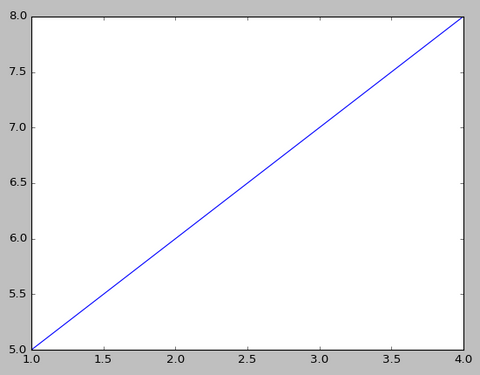
Below shows a simple example wherein we are plotting x against y. In a standard python environment, we must import the matplotlib library and use plt.plot(x,y) to plot a graph. In the Xtralien Scientific Python program, this library is imported already and we can simply use the plot(x,y) command without the plt.
##Standard Python##
import matplotlib as plt
x = [1,2,3,4]
y = [5,6,7,8]
plt.plot(x,y)
##Xtralien Scientific Python###
x = [1,2,3,4]
y = [5,6,7,8]
plot(x,y)
How Do I Use It?
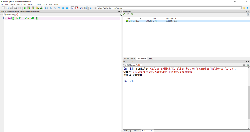
Below shows a screenshot of the Spyder-based programming environment running a simple 'Hello World' example script. Code is written on the left section and the result is displayed in the bottom right. The top right section has tabs which display files, variable values and a help section.
Beginner Tutorials
Python is versatile, intuitive, and easy to learn. It is great for data analysis, instrument control, and systems engineering. These tutorials provide an introduction to Python programming. We will guide you through the basics and show you how to create simple yet powerful scripts.
Printing To The Console
Printing is a simple way for you to display parts of your code.
Commonly, you will use the print function to display the value of variables and how they change as your script runs.
Python provides print among it's standard functions, so it is accessible from anywhere in your code.
If you provide multiple values to the print function, they will be joined together with spaces in between.
As a note, the console is your window through which you can interact with Python whilst it is running. In the Xtralien Scientific Python Distribution this can usually be found in the bottom-right section of the screen.
Printing "Hello World"
To show how simple it is to print to the console in Python, we will print the string "Hello World!" to the console.
print("Hello World!")This is all that is required to print some text to the console.
Printing Results
When you perform a calculation, or would otherwise like to see how a certain variables change throught the execution of your script, you can print this to the console to check the result.
A simple example of this would be to perform a calculation inside a print function call.
print(1 + 1)This should print the number 2 to the console. This shows us that this calculation was performed correctly.
You can print variables as well, which is discussed more thoroughly in the next section.
Printing Headers
When you are making a program you will sometimes want to separate what you print. In Xtralien Scientific Python we have included a function to print headers, called print_header that fulfills this need for you.
print_header("A header")This line will print a header as shown below. The format for the header is centered text with an equal number of hashes on either side to define a clear line.
Variables
Variables are the way that you store values in Python, among other programming languages. Another name for a variable is symbol. Variable assignment is as simple as in mathematics. You store a value in a variable by using the equals symbol (=).
Your first Assignment
Due to Python's resemblence to mathematics, assigning values to variables is as simple as writing an equation.
x = 1We can test this by printing the value of x.
print(x)This would print the value of x to the console, which in this case would be 1.
Assigning a result
Assigning a static value isn't useful by itself, so in most cases you will want to store a result in a variable. In this example we will store the result of a simple addition.
z = 1 + 1This will run the addition and then store the result inside the variable z for later use. We can check this by printing z.
print(z)This will print 2, which is the result of the addition.
Using Variables
As seen before, variables can be used as arguments to functions (more on this later in the functions section). The method by which we use variables is by simply stating them where we wish to use them.
In the above case we provided z as an argument to the print function. In the following example we use the previously defined variable x to create a new variable, y.
y = x * 2This will multiply the value stored in the variable x by 2 and store the result in the variable y.
Updating a value
In Python the assignment of a value to a variable happens after the right-hand-side (RHS) of the assignment is executed. This means that you can update the value of a variable by using the variable in the update.
In the example below we add 1 to the value of z, which we previously defined as 2.
z = z + 1This will run z + 1 and then assign that result to the variable z, overwriting the previous value.
In-place updates
Because these types of updates to variables are common, there is a shorthand for them in Python. These are called in-place updates and they use a modifier on the assignment operator (=). An example of this is a replication of the above example.
z += 1This example will perform exactly as the above example, modifying the value of z by adding 1 and storing the result.
Lists
Lists are a core data structure in Python that are similar to arrays or vectors in other langauges, however they don't have any limitations on length.
A list consists of of a series of any values. Additionally, lists are values themselves, so they can be stored in variables. Lists are mutable, which means they can be modified without needing to create a new copy.
To create a new list you can either use the [] shortcut or use the list() function. Normally, the [] notation is used for clarity.
Lists are good for collecting items as you go through your script. Additionally you can access items inside Lists by using square brackets ([]) after the symbol storing the list. This is called subscript access.
You cannot go out of bounds (try to access outside the list), and attempting to do so will cause an IndexError. The bounds are defined by the length of the list (). Because the indexes in Python start at (The first item is index 0), the maximum index in a List is .
Technical note: For those who are interested, lists are implemented internally as a linked-list data structure. This means that it might be better to use one of numpy's arrays if speed or memory are of the essence.
Creating your first list
It is possible to create lists using two different methods.
One of the methods is to use the list function.
a = list()The other method is to use square brackets.
a = []Both of these methods produce an empty list and are equivalent. This can be checked printing the result of an equality comparison between the two.
print(list() == [])This should print True to the console, indicating that they are equivalent.
Creating a populated list
In the previous example we created a list that was empty. This can be useful if you want to add items as you move through the program, but you may also want to initialise a list with some standard elements. The way that you do this is different for each different type of list creation.
For the list function you need to provide an iterable for the function to turn into a list. This is nominally another list or a tuple, however it can be anything that provides an iterable interface, such as a generator.
a = list((1, 2, 3))The second method, using the [] notation, is simpler and more direct. You simply insert the elements that you wish to be in the list.
a = [1, 2, 3]Both of these methods will create identical lists, which would show [1, 2, 3] if inspected.
Reading items from the list
Reading items from the list is the same as many other languages. In Python it is called subscript access and uses [] after the variable name. Using the example of a = [1, 2, 3, 4] this is shown below.
b = a[0]This would assign b the value 1. This is because 1 is the first element (index 0) of the list stored at variable a.
It is also possible to get a subset of a list, called a slice in Python, using similar syntax. This is done by using the syntax list_variable[start:end] where start and end are both optional. If start is omitted then the index 0 will be used. Likewise, if end is omitted then the length of the list will be used as an index, due to the exclusive nature of end. An example of this would be as follows.
b = a[1:3]This would assign b the value [2, 3] as these are the elements at indexes 1 and 2 respectively.
Adding to the list
You can add to a list by appending items. This is done by providing the element you wish to add to the append method of the list.
a.append(4)This will add a 4 to the end of the list. If the list a is inspected it would display [1, 2, 3, 4].
Removing items
If you need to remove items from a list you can either pop them off of the list or delete them.
If you choose to pop an item from a list you need to use the pop method of the list, providing the index of the item you want to pop from the list. When you pop from a list you get the element you removed.
popped = a.pop(0)In this case we provided the index 0 (the first element) and the first element was removed and returned to us, stored in the variable popped in this case.
If you don't need the popped value then it may be more economical to use the del keyword. This simply deletes whichever value you point to, removing from lists or dictionaries if needed.
del a[0]This code will have the same effect on the list a however it won't return the popped value for you, instead removing it completely.
Troubleshooting
When accessing elements from lists in Python, you will sometimes try to access an element that doesn't exist. If you are getting a single element from a list then you might cause an error to occur. This is an IndexError and it needs to be handled, otherwise your program will terminate.
b = a[10]The example above would cause an IndexError. There is more information on Errors and Exceptions in a later tutorial.
It is worth noting that if you access a slice that is outside the scope of the list then an empty list is returned and no exception is raised.
Strings
Strings are ubiquitous in programming. They can be very useful in explaining what is happening at any given point in a program. At their core a string is simply a series of characters. Often text strings will contain regular words and sentences, however they are not required too.
string_a = "Hello world!"
string_b = "Hlelo wrold!"
In the example above both string_a and string_b are strings although string_b does not contain a correct english sentence.
Creating a string
As seen above, strings can be created by using quotes. In Python both single ' and double " quotes can be used to create strings. The quotes must appear at the beginning and end of the string and must match.
For example, the following are two valid examples of the same string. As you can see, the quotes are the same at the beginning and end of each of the strings.
single_quote = 'Hello World!'
double_quote = "Hello World!"
Once created a string cannot be modified. In this way they are like tuples.
Strings are very useful for communicating with scientific instruments, such as with the Xtralien X100 (discontinued).
It is possible to create new strings by adding strings together. This will result in a new string.
new_string = 'Hello' + ' ' + 'World!' The example above will result in the string 'Hello World!' being assigned to variable new_string.
Accessing a string
Usually a string is accessed all at once, either to compare or to print. However, like a tuple you can access slices of strings. This is done in the same way as tuple and lists.
hello = single_quote[:5]This would assign the value 'Hello' to the variable hello.
Transforming to strings
Most types of value in Python can be transformed into strings using the builtin str function.
string_1 = str(1)The example above assign the value '1' to the variable string_1.
Formatting strings
String formatting is useful when preparing to print values. In other languages, such as C, you prepare string using %-formatting. You can also format like this in Python, like below.
formatted_string = 'Hello %s' % 'World'This will assign the value 'Hello World' to the variable formatted_string. This is because 'World' is inserted in place of %s.
With new versions of Python, the string type has gained a format method, which can be used for easier formatting. When using this method the %-formats are replaced with {} and the str version of each type is used instead.
The example above could be rewritten using the format method as below.
formatted_string = 'Hello {}'.format('World')This would provide the same result as the first example and it is more pythonic because it doesn’t rely on any types.
Tuples
Tuples are similar to lists in Python in all except they cannot be modified once set. The only way to change a set stored in a variable is to overwrite the the variable with a new set with new elements.
Creating tuples
Creating tuples is similar to creating lists. We can simply use the () notation to create a tuple. This is analagous to the [] notation for lists. There is one additional difference however, in that tuples cannot have a length of \(0\).
A further caveat is that tuples of length \(1\) must also contain a comma. This is because brackets surrounding values are sometimes used to to define a scope when calculating values to adhere to correct order of operations.
a = (1,)The above example will assign a tuple containing only the value 1 to the variable a. Creating a that has a length larger than one is intuitive knowing the above.
a = (1, 2)The example above shows how to create a tuple of length \(2\) containing the values 1 and 2.
Accessing tuples
Accessing tuples is the same as accessing lists, including creating slices. This means that in terms of accessing elements in each, they are interchangable.
If we have the tuple a.
a = (1, 2, 3, 4)Then, as in lists section, we can access single elements of the tuple.
b = a[0]This would set b to the value 1.
Likewise, we can take a slice of a tuple.
b = a[1:3]This would set b to the value of (2, 3).
Note: A slice is of an iterable is usually of the same type as the origin. e.g a slice of a list is a list and a slice of a tuple is a tuple.
Dictionaries
Dictionaries are a core data construct in Python. They work by using a key to map to a value. This key can be any unique Python value and the value can also be any unique Python value. However, typically strings are used as keys due to their readability.
Creating a dictionary
To create any dictionary you use {}, where the curly braces denote the beginning and end of the dictionary, like the square brackets for a list.
a = {}The example above would create an empty dictionary. To populate a dictionary on creation you use a pattern like below.
a = {
key: value,
key: value
}
As you can see above, multiple entries are separated by a comma ,, with each entry consisting of a key and value.
A use case for a dictionary might be something like a small local database. In the example below a few periodic elements are mapped from their symbol to their name in English.
periodic_table = {
'H': 'Hydrogen',
'He': 'Helium',
'Fe': 'Iron'
}
Reading a dictionary
To read from a dictionary you use a similar subscript style to that of lists. Continuing from the above example, we can get read the name of the element with H as it’s symbol. We do this by providing the key that we want to look up.
element_name = periodic_table['H']The above example will load the value stored at key 'H' in the dictionary periodic_table. In this case that means that 'Hydrogen' is stored in the variable element_name.
In the case that the key doesn’t exist in the dictionary you will get a KeyError. This is similar to an IndexError that you get when you try to access a nonexistent list element. However, with dictionaries you can use the get method to return a default in the case that the key doesn’t exist.
element_name = periodic_table.get('H', "default value")The above will store 'Hydrogen' in the variable element_name. We can also choose to search for a key that doesn’t exist, like 'Xe'.
element_name = periodic_table.get('Xe', "default value")This will store the value "default value" in the variable element_name. This pattern of accessing databases is good for settings because you can set a default for any optional value.
Note: It is not possible to use slices with dictionaries
Updating a dictionary
If you wish to update a dictionary to contain a certain key-value then you can set the value directly.
periodic_table['Xe'] = "Xenon"The above example will set the key 'Xe' in the dictionary periodic_table to the value "Xenon".
In cases where you want to set multiple values of a dictionary you have two options. You can either set each key separately as above, or you can update the dictionary using another dictionary.
periodic_table.update({
'C': 'Carbon',
'O': 'Oxygen'
})
If any of the keys already exist in the periodic_table dictionary then the new values are the ones stored, overwriting the old values. Any keys that don’t exist are created with the new values.
Deleting from a dictionary
To remove any elements from a dictionary you need to del the key from the dictionary. This will remove the key and the value from the dictionary.
del period_table['O']The above example will remove the element with a key of 'O' from the dictionary. If the key doesn’t exist this will cause a KeyError, as if you were accessing the value at the key.
Conditionals
Conditions are how decisions are made. In Python we can use conditions to change what our program does. In programming this is usually represented by a boolean, i.e. a True or a False value.
Booleans
Booleans are a type of value that is either truthy or falsey. This goes along with the two states of truth that are used in the real world.
In Python these are represented with the True and False values. Most non-boolean types can also be seen as directly boolean.
For lists, tuples and strings they are seen to be falsey when their length is \(0\) and truthy otherwise.
For numbers, \(0\) is considered falsey and any other number is truthy.
Boolean operators
To coerce a boolean value from non-boolean values, such as strings or numbers you normally perform a test that you want to check for. This may be testing wether a number is in a certain range.
x = 5
y = 1 < x < 10
In the example above y now contains the Boolean result of the test (True).
The Boolean operators that can be used are as follows.
| Operator | Name | Example |
|---|---|---|
< |
Less than | a < 5 |
<= |
Less than or equal to | a <= 5 |
>= |
Greater than or equal to | a >= 1 |
> |
Greater than | a > 1 |
== |
Equal to | a == 1 |
!= |
Not Equal to | a != 2 |
!/not
|
Not (Inverse of Boolean representation) | !a |
In the case of the ! operator, this get the Boolean value of the variable and then return the opposie of that.
It is also possible to combine the reults of comparisons into a single result using and and or.
| Left | Operator | Right | Result |
|---|---|---|---|
True |
and |
True |
True |
True |
and |
False |
False |
False |
and |
True |
False |
False |
and |
False |
False |
True |
or |
True |
True |
True |
or |
False |
True |
False |
or |
True |
True |
False |
or |
False |
False |
If
The simplest conditional in Python is the if structure. At it’s simplest this will create a boolean from the expression given and check if the value is either True or False.
The value of this expression is evaluated and used to decide wether the code inside the if statement is run.
value = True
if value:
# Code to run if value is truthy
print("Value evaluated to True")
The above example will print Value evaluated to True to the console because value is currently set to True. If value was set to a falsey value then none of the above code would be run.
else
Else is an extension to if, and can be used as a default. This is analagous to if 1 do 2, otherwise do 3
. By using this structure you can provide defaults, or some alternative code to run that should only run if the condition (value) is falsey.
value = False
if value:
# Never called because of False
print("Value is truthy")
else:
# Called because value is False
print("Value is falsey")
The example above shows that when the value provided to the if statement is falsey then the else will run.
elif
Python provides a third keyword that is a mixture of both if and else. You use the elif keyword when you want to check for another condition. You might do this to check if an element is in a certain range.
An example of this would be checking if any roots exist in a quadratic equation.
The part of the equation we need to check this is as follows.
a = 2
b = 4
c = 1
n = (b ** 2) - (4 * a * c)
if n > 0:
print("There are 2 real roots")
elif n == 0:
print("There is a single real root")
else:
print("There are no real roots")
The example above shows a simple program that can determine the number of real roots in a quadtratic. The elif keyword is used to check another condition. This will only be tested if the first case evaluates as falsey. If this case also evaluates as falsey then the final case (the else will run). This is similar to other programming languages, however in Python there is no concept of a switch/case so using if, elif and else are the only methods of making decisions.
Assigning values using or
Sometimes you will want to set a vaariable to a certain value on a condition. You can either do this by using a standard if/elif/else like below.
if some_value:
value = 1
else:
value = 2
However this is quite a large structure. Luckily, in Python it is possible to compress this to a single line like below.
value = 1 if some_value else 2This means that you can do short optional assignments without having to write more code than is needed. Additionally, it is arguably clearer to read the second version than the first.
Taking this further if you wanted to assign a value contingent on it being truthy, then you could write the following.
value = some_value if some_value else 1The above example would check that some_value is truthy and if so then value would be assigned the value that is currently held in some_value. If not then the value 1 would be stored in value.
Due to the common appearance of this pattern there is a shorter way to do this in Python.
value = some_value or 1The example above is essentially the same as the previous example, checking some_value to ensure it is truthy and then setting the value as appropriate. The additional benefit is that this can be easily extended to provide cascading checks.
value = some_value or some_other_value or 1The above example will check each value to ensure it is truthy and move onto the next value until a truthy value is found, or it reaches the end of the assignment. Then the appropriate value is set.
Loops
When programming you will often need to run a section of code or perform a certain series of options a number of times.
In Python you can do this using different types of loops. Nominally you will use both the for and while loops, and both are explained below.
for loops
for loops are a common type of loop in Python.
When using the for loop in Python you use the format for element in iterable. This is the only form that a for loop takes. It will cycle through each element in an interable and run the code inside the loop scope (The additional indentation after the loop).
iterable = [1, 2, 3]
for element in iterable:
# Perform operations on the element
print(element)
for loops exist to process data rather than perform a set number of loops, although this behaviour can be forced by using the range function, which produces a list of a set size. A simple example of this can be seen below.
for i in range(10):
print(i)
This example will print \(10\) numbers, from \(0\) to \(9\) inclusive. While this example is not particulary useful you can use loops like this alongside the built-in enumerate function. This allows you to move through data with an index.
data = [1, 2, 3, 1, 2, 3]
for index, value in enumerate(data):
data[index] = value * 2
This example shows the power that you gain by using for with the enumerate function. Using the above you can process and update a list of data.
while loops
while loops are slightly simpler because they are based on condition. Every time this loop starts a cycle there is a check to ensure that the loop should run. If this check is truthy then the loop will run the code inside the while loop.
While loops are useful when monitoring systems due to their intrinsic function of inspecting a condition.
i = 0
while i < 10:
print(i)
i += 1
The example is similar to the example seen in the for loop section. The output will also be the same, printing the numbers \(0\) to \(9\) inclusive.
Breaking out
It is sometimes useful to change the flow of loops or break out of them entirely. to do this there are two useful keywords, continue and break. The continue keyword ends the current cycle of the loop and moves back to checking the condition, resetting the loop.
i = 0
while i < 10:
i += 1
if i % 2 == 0:
continue
print("i is odd")
The above example uses this behaviour to only print when numbers are odd, even though the loop will execute 10 times.
Conversely, The break keyword will stop the loop in place and then exit the loop, not returning to the start. Commonly this is used with a while loop to perform some action forever, unless a specific condition is met.
while True:
result = test_something()
if result == 0:
break
This will continue running until the function test_something returns 0.
Both of the above constructs are useful when developing an application that needs to repeat something for a number or times.
Functions
Functions are a way of grouping actions and processes, whilst additionally providing a reusable interface. Although code needs to be designed to take advantage of this reusability, it is often useful to do so to reduce total development time.
Functions also provide a standardised interface to hardware and other software. This allows you to change the underlying mechanics of the function without having to change the interface that you use to access it.
Functions can also be used in conjunction with classes, which are user-defined types. When used in this way functions are referred to as methods.
A useful anaolgy is that well-designed functions often act as black boxes. This is because they should provide a consistent interface, with anything involved concealed within the function.
Defining a function
When creating a function you are defining what it does. This is why when you define a function you use the def keyword.
def function():
pass
The definition of the function function uses a new keyword pass, which tells Python to do nothing. This is useful when starting to structure your function definitions. When indenting you can use pass to keep your code correct when you don’t know what the final definition will be. It is a useful placeholder.
The example above does one thing only. It defines a function stored in the variable function. This function takes to arguments and returns no value.
One example of when you may want a function that has no input or output is when the function does a very specific job.
def print_header():
print("HEADER")
The above function has limited functionality but shows how a function contains instructions on further actions to take. Unfortunately these functions take no arguments and so have limited capability. The next sections alleviate this problem.
Returning from functions
Most of the time when using functions you will want to return a value from a function. In Python you can only return a single value from a function, although this can be a tuple, allowing you to return as many values as you wish.
To return values from functions in Python you use the return keyword. When used, this will stop the function where it is and return the specified value.
Note: you do not need to specify a return value, allowing return to be used to exit a function.
def get_random_percentage():
return random() * 100
In Python the random function is from the random module, and provides a number betwwen 0 and 1 as a result. The example above will simply take this value and multiply it by 100 to get a value between 0 and 100.
It is also possible to use arguments to create a function that acts on the input and returns a result based on the inputs.
Taking arguments
In Python you can choose to take arguments in your function by naming the arguments that you want.
def miles_to_km(distance):
return distance * 1.61
miles = 2
km = miles_to_km(miles)
print("There are {} km in {} miles".format(km, miles))
In the example above the variable distance is ‘bound’ to the argument passed. In the case above the value 2 is bound, meaning that for the duration of the function, the variable distance will contain the value 2. The miles_to_km function will then multiply the provided distance by 1.61 and return the result. This example will print There are 3.22 km in 2 miles to the console.
Default arguments
It is possible to provide default arguments to functions so that not all of the arguments need to be provided every time that the function is used.
One example of a function that uses default arguments is the range function. This function will have default values for start and step of 0 and 1 respectively. It is possible to override this simply by supplying the other arguments.
start = 0
end = 10
step = 1
range(start, end, step)
range(end)
Because the arguments are the same as the defaults in this case the result will be an iterator containing the integers from 0 to 9 inclusive.
To define your own function with default arguments you can use syntax like below.
def print_name(name="John"):
print("Hello", name)
print_name()
print_name("Jenny")
The above example shows how optional arguments can be used to provide alternatives for when an argument is not provided. In this case, when the function is called the first time, without any arguments the string Hello John will be printed. This is because the variable name defaults to the string John. In the second call of the function the name "Jenny" is provided. This will override the value for name, meaning that Hello Jenny will be printed to the console.
Scopes
Scoping in Python refers to variables. There are two scope ‘levels’, global and local. By default you can only read the local scope. The global level is where most of your functions exist. The local scope usually only exists when you are inside a function, and is unique to a specific instance of the function execution.
When you are outside any function the global scope is the same as the local scope, however when you enter a function then a new local scope is created. Any assignments in this local scope are not applied to the global scope, and are lost when the function ends. An example of this is below.
# In global scope
x = 1
def set_x():
# Created a new local scope
x = 2
print("function x:", x)
# Destroy local scope
print("x:", x)
set_x()
print("x:", x)
The above example shows how scopes are created and destroyed as you enter and leave functions. Both of the print statements around the set_x function call will print x: 1. This is because that is the value of x in the global scope. The local scope makes its own x and assigns that value to 2. However, as the function finishes the local scope gets destroyed.
When access to the global scope is required from inside a function it is possible to declare that you require access to that variable. To do this you simply need to declare that you want to use the variable before you attempt to use it. Rewriting the example above we can see how access to a variable in the global scope can be achieved.
# In global scope
x = 1
def set_x():
# Specify that we are using the global x
global x
# Created a new local scope
x = 2
print("function x:", x)
# Destroy local scope
print("x:", x)
set_x()
print("x:", x)
This new example will modify the global variable x and replace the value with the value 2. In this case the last print statement will show that the value of x has changed from 1, as initially set, to 2.
Intermediate Python Tutorials
These tutorials cover slightly more advanced topics, which you can use to create functional and powerful scripts.
Imports
When writing programs well organised code can be key to understanding the underlying processes of your code. Because of this it is often useful to split your program across files dependant on the purpose of each part of code.
Structure preface
Before importing a module it is worthwhile knowing how a typical project is structured. When you import a module, Python starts to search in 2 places.
- The folder containing the running file
- The main Python library directory (this is inside Xtralien Scientific Python)
This search will end as soon as a match for the module is found.
When importing the module, any nested import statements will also be run, which is why it can be useful to split related functions and classes into functions.
common/
functions.py
classes.py
main.py
The above directory structure would allow the main body of code to be placed in main.py, which could import common functions from common/functions.py by running import common.functions. This way common.classes is not included, which reduces the size of the program in memory, speeding up the programs execution.
Note: It is also recommended that python files and functions are kept short and concise to enable greater comprehension of their contents and function.
Importing a module
To use another file, or module in your program you need to import your module. Importing a module uses the import keyword.
import numpyThe above line will search for the numpy module and, if available, store the contents of the module into the variable numpy.
Using as
It is possible to set the name of the import when importing by using the as keyword. This is similar to importing into the current file and then assigning the module to a new variable name.
Importing from a module
Most of the time you will not need everything from a module. In these cases you can make use of the from keyword to import a selection of the module directly into the current module.
from numpy import array, randomThe line above is relatively simple, and it will load both array and random from numpy to allow them to be used in this module.
Import everything
To import all members of a module you can use the * operator.
from numpy import *The line above will import everything that from numpy, such as random and array.
Note: Although this is useful for brevity it is often harder to fix any issues using this method.
Import Errors
If the module you want to import does not exist then using import to import it will cause an ImportError to be raised. Using techniques such as the try/except structure it is possible to check for a module and import an alternative if needed.
try:
import numpy
except ImportError:
 import my_numpy as numpy
The above example will attempt to import the numpy module, failing which the my_numpy module will attempt to load. This allows default libraries to be used, enabling greater compatability across different systems.
This is useful if you develop programs that run on different systems, where not all of the optimised libraries may be available. Writing programs this way lets you get the additional performance when you can, and still have a functioning program otherwise.
Numpy
Numpy is a Python Module that enables accelerated Numerical manipulation in Python. The method by which this is achieved is by using C and Fortran for the internals of the module.
This use of low-level code can increase the performance of numerical operations by multiple orders of magnitude. This speed increase can be useful for many applications, including data/signal analysis.
Arrays
Arrays are one of the key parts of numpy. These arrays are like those found in C, and are the reason for the large speed-boost from Numpy.
list_1 = range(10000)
list_2 = range(10000)
list_3 = []

print("1:", list_3)

for x, y in zip(list_1, list_2):
list_3.append(x + y)

print("2:", list_3)
The example above shows a typical Python method of adding together the numbers in two lists. On a typical instance of Python 3 this can take \(1.7ms\) per run.
from numpy import array, arange
list_1 = arange(10000)
list_2 = arange(10000)
list_3 = list_1 + list_2

print(list_3)
Note: The examples above import from the
numpymodule, however this is done for you in Xtralien Scientific Python. It is explicitly listed here for completeness.
The above example shows how fast numpy arrays can be. When run in the same Python instance as the previous code, each invocation lasts for approximately \(17µs\) (\(0.017ms\)) per invocation. This makes numpy approximately \(100\times\) faster than native Python lists for processing datasets.
The difference is that the second example uses numpy’s native array methods instead of Pythons range and list interfaces.
One other key point to notice is that the numpy code uses a more intuitive list_1 + list_2 instead of a for loop. This hides complexity and allows for more clarity in the algorithms being developed, rather than forcing the user to focus on low-level details.
Broadcasting
Numpy arrays also have an ability to ‘broadcast’ operations. This means that even using Python methods and operators, such as + will be made faster by applying to every element of the array at once.
number_array = arange(10000)
number_array += 10000
By the finish of the above example, number_array will contain the integers from 10000 to 19999 inclusive. This is useful to enable operations such as centering around the mean of data.
Plotting with Matplotlib
In Python you typically plot data using the matplotlib library. This tutorial shows you how to make a simple plot and customise it for presentation.
Your first plot
matplotlib is a library that allows for easy plotting of data in Python.
x = [1, 2, 3, 4, 5]
y = [3, 5, 7, 8, 9]
figure()
plot(x, y)
show()
Note:
figure()andshow()are optional in the Xtralien Scientific Python, however they are recommended as they are explicit and can show you where your figure starts and ends.
The above example shows the most common plot, the line plot. the plot function takes a list of x values, and a list of y values. These two lists should be equal in length as they will be matched to each other when plotting, e.g. (1, 3), (2, 5).
The figure function defines the start of a new figure
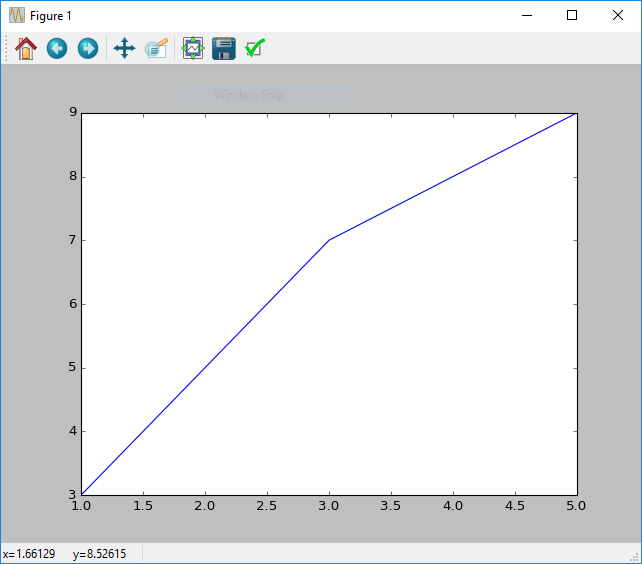
By default the plot will extend to the beginning and end of the plot.
Multiple plots
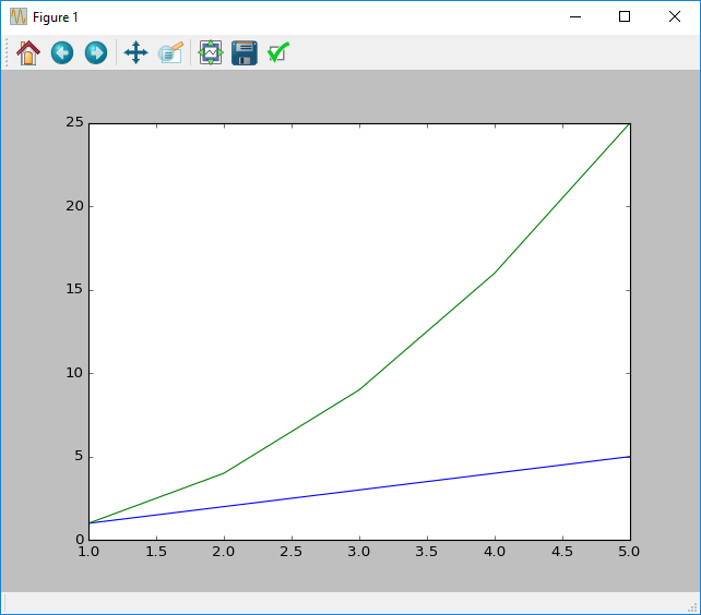
Sometimes it is useful to plot multiple lines on a graph to compare series of data. Because matplotlib stores previous graphs until you clear the figure (using clf), it is possible to plot multiple graphs on the same figure by repeating the plot command.
# x values
x = [1, 2, 3, 4, 5]
# First y series
y1 = [1, 2, 3, 4, 5]
# Second y series
y2 = [1, 4, 9, 16, 25]
# Plot everything
figure()
plot(x, y1)
plot(x, y2)
show()
The code above will produce a plot with two lines for each of the different plots. These are different colours to easily differentiate the two.
Note: The x does not need to be shared as the graph will expand to fit the largest plot. However the x and y lists for each indiviual
plotneed to be the same size.
Customising your plot
It is possible to further customise your plot to make it easier to interpret, or to stylise your results.
Adding a title
Adding a title is useful when creating figures that you plan to publish, or simply to explain at a glance what the plot shows. The function that matplotlib contains to do this is title. To use title you just pass the string you wish to use as the title.
x = [1, 2, 3, 4, 5]
y = [3, 5, 7, 8, 9]
figure()
plot(x, y)
title("2x + 1")
show()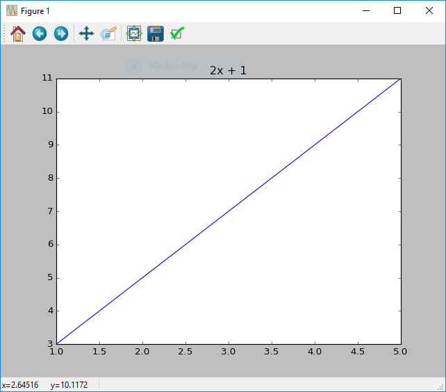
2x + 1.Adding axis labels
To add a label to an axis you can use the xlabel and ylabel functions in matplotlib. These will add a labels to each relevant axis. Both of these functions take a string that will be used as the relevant axis label.
x = [1, 2, 3, 4, 5]
y = [3, 5, 7, 9, 11]
figure()
plot(x, y)
xlabel('x')
ylabel('y')
show()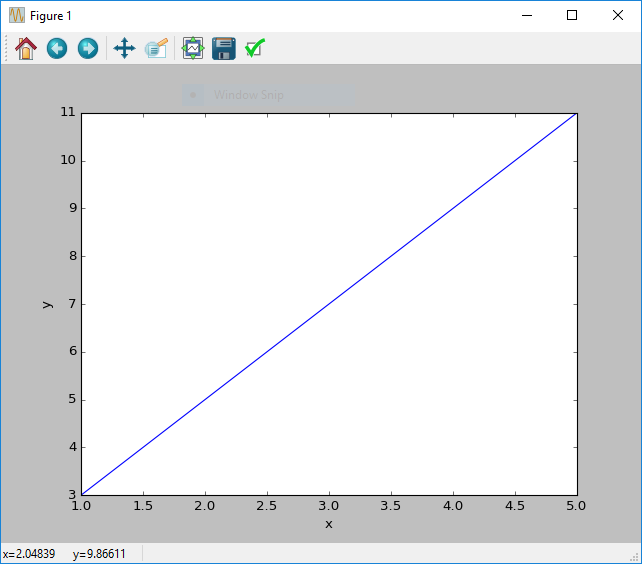
Adding a grid
To add a grid in matplotlib you simply need to use the grid function. This function takes two optional arguments, major and minor, which refer to the major and minor gridlines respectively.
By default major is True and minor is False, resulting in a grid that shows the major gridlines.
x = [1, 2, 3, 4, 5]
y = [3, 5, 7, 9, 11]
figure()
plot(x, y)
grid(major=True, minor=False)
show()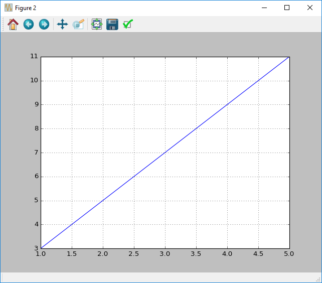
Changing Scale
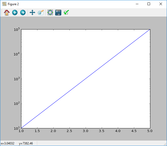
When plotting using matplotlib most plots will either use a linear scale, or logarithmic scale. Depending on the effect that you are investigating both may be of interest.
The easiest method of changing the scale is through the use of the xscale and yscale functions. Both work similarily and take a string as an argument.
To change the y axis scale to linear mode you would use yscale('linear'), and to change the scale to a logarithmic scale you would use yscale('log').
x = [1, 2, 3, 4, 5]
y = [1e1, 1e2, 1e3, 1e4, 1e5]
# Linear plot
figure()
plot(x, y)
yscale('linear')
show()
#
figure()
plot(x, y)
yscale('log')
show()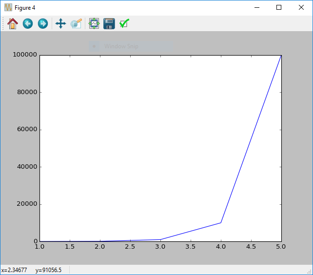
Changing axis limits
Axis limits are customisable for each plot, and can be changed by providing the minimum and maximum values for each of the limits respectively.
You can use the xlim and ylim functions for this purpose. An example of when you would want to do this is if you wish to focus on a specific point, such as a point of intersection between two lines.
# x values
x = [1, 2, 3, 4, 5]
# First y series
y1 = [1, 2, 3, 4, 5]
# Second y series
y2 = [1, 4, 9, 16, 25]
# Plot everything
figure()
plot(x, y1)
plot(x, y2)
# Set the limits
xlim(2, 3)
ylim(5, 6)
# Show the plot
show()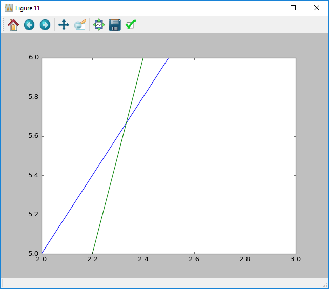
Creating a legend
It is possible to create a legend in matplotlib by using the legend function. This function creates a legend in a corner of the plot.
To label this legend you need to supply a label to every plot that you create. label is a string, and will appear next to the line in the legend.
# x values
x = [1, 2, 3, 4, 5]
# First y series
y1 = [1, 2, 3, 4, 5]
# Second y series
y2 = [1, 4, 9, 16, 25]
# Plot everything
figure()
plot(x, y1, label="2x + 1")
plot(x, y2, label="x*x")
show()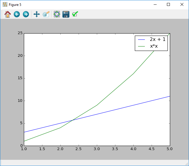
Files
File storage is central to many applications as some application state or configuration must often be preserved to be read, written or logged.
open files
In Python the concept of files is heavily used, borrowed from the UNIX family of operating systems. This means that a file must be opened to be read or written to.
The method to do this is by using the open function. This function takes one required parameter filename, and one optional parameter mode. This filename can either be relative or explicit:
- A relative file will be opened from the location of the file that is running.
- A full path is the full path from the root of the device. e.g.
C:\\on Windows.
Note: When using windows, the
\character will need to be escaped (\\) because\is the escape character.
Modes
When opening files a mode can be supplied to allow writing or appending to the file.
| Mode modifier | Description |
|---|---|
r |
Read mode, open file for reading |
a |
Append mode, add data to a file without removing any |
w |
Write mode, overwrite the file and open for writing |
+ |
Open the file for both reading and writing |
b |
Binary mode, used to write and read bytes rather than strings |
Both + and b are used with another mode. If no mode is supplied then r is used as the default value.
Path handling
To handle multi-platform issues, and enable sharing of code it is recommended that file paths use the os.path module.
Note: The
osmodule also contains utilities for checking if files exist and are readable, however for this simple tutorial we will just concern ourselves withos.path
from os import path
some_file_path = path.join('C:', 'Users', 'YOUR_NAME', 'some_file.txt')
The above example would store the string 'C:\\Users\\YOUR_NAME\\some_file.txt' in the variable some_file_path on Windows.
The os.path.join function joins the arguments to the function similar to string formatting. This makes sure that the paths are correct in your strings.
Error handling
OSError is the most common exception that file access may cause. This is usually caused when a file cannot be opened. It is common to see file-handling enclosed within a try/except block to ensure incorrect file access will not cause any data loss.
try:
f = open('filename.txt')
# Use the file
except OSError:
print("An error occurred opening the file")
The example above highlights this usage. The main body of the code would be contained in the try block. Alternatively it is possible to use the with keyword to handle this automatically.
with open('filename.txt') as f:
# Use the file
This has the same effect as the previous example, with the main content of the code\ located inside the with block. This typically looks cleaner and is more understandable.
CSV files
CSV (Comma Separated Value) files are one of the many open standards that have become useful to many data processing tasks.
The CSV filetype is powerful due to two main features.
- The standard is simple and human-readable.
- The standard is open and can be easily read by many programs (including Microsoft Excel).
Whilst there is the csv python module included in Python already, we have added two functions to our Xtralien Scientific Python distribution that allow easy handling of numpy arrays.
array_to_csv is one of these provided functions, which takes a numpy array and a filename. This is called like below.
array_to_csv(numpy_array, 'filename.csv')This would save the array stored in numpy_array into the file filename.csv.
There is a counterpart to this which is the load_csv function, which will load a csv from the provided filename argument.
data = load_csv(`filename.csv')The example above highlights this usage. data will be allocated a numpy array containing the data found inside 'filename.csv'.
Exceptions
Exceptions are used in Python to express when an error has occurred. Usually they will provide a detailed explanation of where the program stopped. Additionally the exception may explain why the program has failed, although this is not always possible.
Creating Exceptions
To create an exception you raise an Exception. To do this you use the raise keyword alongside the error that you want. To raise a generic exception you can use the Exception class. The Exception class is used as the root of all Exceptions, meaning that most exceptions ‘wrap’ the Exception class.
raise Exception("A generic Error")In the above exception you can see that we have used the raise keyword to raise the exception Exception, with a message of "A generic Error". This message is provided to assist in debugging your program if it breaks. Because this happens as the program is running you can dynamically create this message using techniques like string formatting. An example of this can be seen below.
raise Exception("Error code: {}".format(404))Handling Exceptions
Often you will want to ‘handle’ exceptions so that your script doesn’t break halfway through and ruin what you have prepared. To add in this error handling you need to make use of the try/except structure.
try:
pass # Do something that might break here
except KeyError as e:
print("Handled KeyError", e)
except IOError:
print("Handled IOError")
except:
print("Exception handled, resuming normal operation")
print("Normal operation")
The example above shows how you can handle exceptions in different ways. In the try section you should put your breaking code.
The first one of these is the except KeyError as e. This will check that the exception is a KeyError (the error for accessing a missing dictionary key), and then store the exception in e if it is.
The second handler is except IOError, which will check if the exception is an IOError (The error code for trying to access files that don’t exist). This one will not store the exception, but just stop it from propogating further. This is useful if you need to retry something.
Finally there is except by itself, which is shorthand for except Exception, due to Exception being the base exception class. This is the default for any exceptions that haven’t already been handled. Similar to the else in an if/else structure.
After any errors have been handled the program will continue normal execution. In this case, this means that Normal Operation will be printed to the console.
Note: When an exception occurs, any code in the same block after the exception will not execute.
Defining new exceptions
Defining new exceptions is simple, even without knowing how to define new classes.
class MyNewError(Exception):
pass
The example above will define a new error MyNewError that is based on Exception. Because the definition consists of just the pass keyword no special behaviour will be implemented.
To raise this error we can use use the first example.
raise MyNewError("An error occurred")To catch your exception, but no other exception we can also use code from above.
try:
raise MyNewError("An error occurred")
except MyNewError:
print("A MyNewError occurred")
The above example shows how you can define an error and handle instances of this error.
Module List
Xtralien Scientific Python contains a list of handpicked modules that assist you in designing applications and experiments. To aid development of experiments using Xtralien Hardware products we also created a library to interface with them in a more Pythonic way. You can read more about this in our tutorials, but at the core of it this is the easiest way to build any experiments that our hardware is capable of running. Details and licensing information on these products is provided below.
Numpy
Numpy is a module that is used in a large number of other modules because of its speed in processing large matrices. This is useful in a number of scientific and computing fields, such as image processing or manipulation. A many libraries to perform such functionality rely heavily on numpy.
Matplotlib
Matplotlib is a library that is used in Python to easily create a display various forms of charts and graphs. Plotting is as simple as calling plot(x_values, y_values) in most cases. More can be seen in our tutorials on matplotlib.
SciPy
SciPy is a library that contains some specialist functions that can be used scientific experimentation. Numpy is used as a base for many of these functions.
PySerial
PySerial is a module through which you can connect to serial-based devices. This includes the Xtralien Hardware, but also covers many other scientific pieces of hardware. The communication happens at a low level and uses byte strings.
PyVISA
PyVisa is a Python module that can be used to communicate with any devices using the VISA communication standard, such as Any devices manufactured by Keithley.
Spyder
Spyder is both a GUI integrated development environment, as well as a framework that contains all of the needed components. As we have used Spyder as a base we have also used the Spyder module.